by Möbius et al.
Abstract: The Interstellar Boundary Explorer (IBEX) samples the interstellar neutral (ISN) gas flow of several species every year from December through late March when the Earth moves into the incoming flow. The first quantitative analyses of these data resulted in a narrow tube in four-dimensional interstellar parameter space, which couples speed, flow latitude, flow longitude, and temperature, and center values with approximately 3° larger longitude and 3 km s-1 lower speed, but with temperature similar to that obtained from observations by the Ulysses spacecraft. IBEX has now recorded six years of ISN flow observations, providing a large database over increasing solar activity and using varying viewing strategies. In this paper, we evaluate systematic effects that are important for the ISN flow vector and temperature determination. We find that all models in use return ISN parameters well within the observational uncertainties and that the derived ISN flow direction is resilient against uncertainties in the ionization rate. We establish observationally an effective IBEX-Lo pointing uncertainty of ±0.18° in spin angle and confirm an uncertainty of ±0.1° in longitude. We also show that the IBEX viewing strategy with different spin-axis orientations minimizes the impact of several systematic uncertainties, and thus improves the robustness of the measurement. The Helium Warm Breeze has likely contributed substantially to the somewhat different center values of the ISN flow vector. By separating the flow vector and temperature determination, we can mitigate these effects on the analysis, which returns an ISN flow vector very close to the Ulysses results, but with a substantially higher temperature. Due to coupling with the ISN flow speed along the ISN parameter tube, we provide the temperature TVISN∞ = 8710 +440/ -680 K for VISN∞ = 26 km s-1 for comparison, where most of the uncertainty is systematic and likely due to the presence of the Warm Breeze.
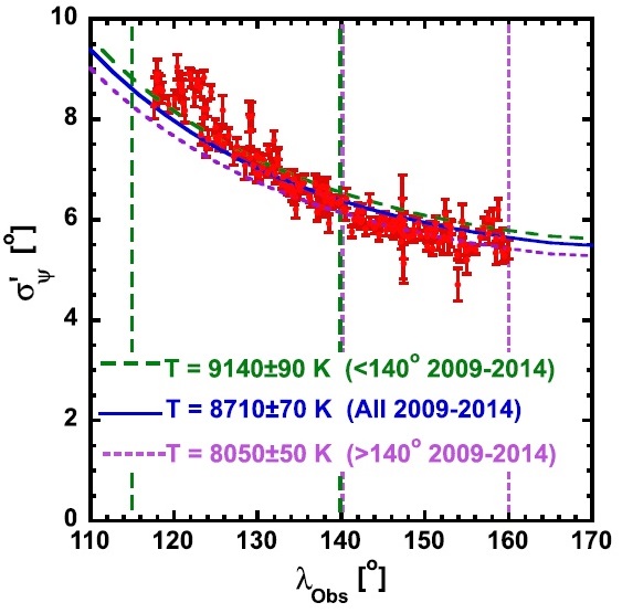
The IBEX Data Products used for the ISN temperature analysis presented in Figure 9 and Table 2 of Möbius et al. (2015). There is one worksheet for each ISN season that was analyzed (2009 – 2014). Shown are 5 data points for each IBEX Orbit arc under investigation. Based on the Start and Stop Times in the “ISN List” the Histogram Corrected Counts of ISN flow distributions in the Level 3 Data of this Release were accumulated for each Orbit arc and then subdivided into 5 time intervals of equal accumulation time.
The data consist of:
- Year Ecl Long: Center Ecliptic Longitude of each time bin in degrees
The center longitude refers to the center time of each of the 5 time intervals. Some intervals may consist of smaller discontiguous intervals. In any case the actual accumulation times are subdivided equally between the left and right half of the time interval.- Year Sigma: Width of angular distribution
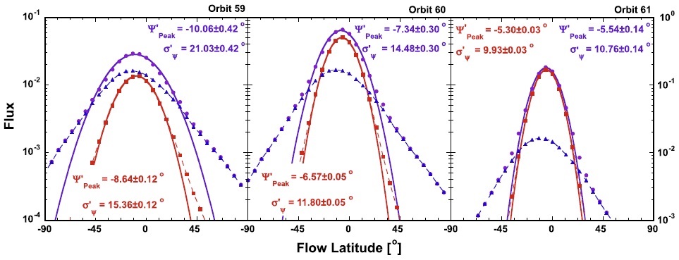
Sigma width of a Gaussian that fit to the angular distribution, including a convolution of the IBEX-Lo collimator function- Year ∆Sigma: Fit uncertainty of angular distribution
Purely statistical uncertainty from the fit routineSigma and ∆Sigma were obtained through a Maximum Likelihood Fit of a Gaussian to the observed angular distributions of the Histogram Corrected Counts of the ISN Flow, after convoluting the collimator function over the Gaussian.
Before using the data for the analysis, two additional corrections were applied:
1) For the analysis the Counts were accumulated in 6 degree bins. The difference between an angular distribution at highest angular resolution and 6o binning was not implemented in the fit, but corrected for afterwards in the second set of columns (E – G). The necessary correction factors had been obtained as a quadratic fit to the difference between model Gaussians with Sigma width of 5 degree< – 10 degree when analyzed with 1 degree and 6 degree binning. The fit parameters (m0, m1, m2) are shown above the columns with the corrected Sigma widths.
2) The distributions for years 2009 through 2012 were corrected for small flux dependent data transfer suppression between IBEX-Lo and CEU (that is described in Möbius et al. (2015) and Swaczyna et al. (2015)). We corrected all width for an average increase of 1.5% (equivalent to an apparent temperature increase of 3%). 1013 and 2014 data do not show the suppression and thus do not need a correction.
2012 through 2014 data are also subdivided into ascending (a) and descending (b) arcs for the separate analysis shown in Table 2.